In this blog I will explore some geospatial analysis and visualization using the Flickr Data found in the Creative Commons 100M Images/Video. In particular I will demonstrate Paul Evangelista’s Point Density plotting package as well as the leaflet interactive map package. I originally created this as part of an RStudio Presentation that I presented at the Army’s Data Science Center of Education (DSCOE). I’ve extracted this part of it for a blog post.

Introducing Yahoo Flickr Creative Commons 100M Images/Video Data

The Yahoo Flickr Creative Commons 100M Data Set is a large dataset that was introduced to the computer vision and multimedia research community. Is is a great data set to conduct research on photo data, video data, or just big data in general. Below are some of the dataset attributes:

• 100 Million media objects (picture and Video)
• Contains objects from 2004 (Flickr inception) through 2014
• 99.2M Photos and 0.8M Video
• Metadata available
• 69M objects contain tags
• ~50% of objects are geotagged
• Available on AWS. See Yahoo Link

Plotting point density of Flickr Data in Australia

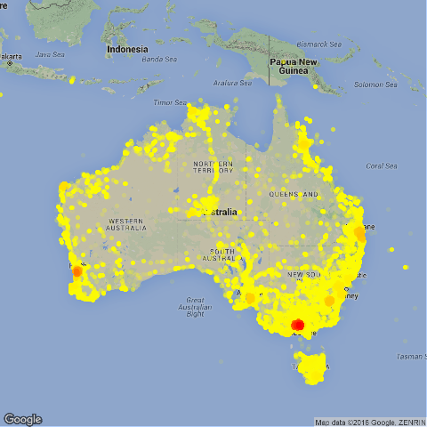
We will start by illustrating how to use Paul Evangelista’s Point Density algorithm to generate a density map of the data in Australia. Paul created this algorithm in perl to assist with point data for the Department of Defense, and I assisted him in translating it to the R Programming Language. I will go into more depth on this algorithm in a separate blog post. I illustrate it’s use below with the Australia Flickr Data:

Code for creating Point Density Plot of Australia:

aus.density<-pointdensity(aus.subset,lat_col="lat",lon_col="lon",grid_size=20,radius=50)
map_base <- qmap('Australia', zoom = 4, darken=0.2) 
map_base + geom_point(aes(x = lon, y = lat, colour = count,alpha=count), 
    shape = 16, size = 2, data = aus.density) + 
    scale_colour_gradient(low = "yellow", high = "red") 

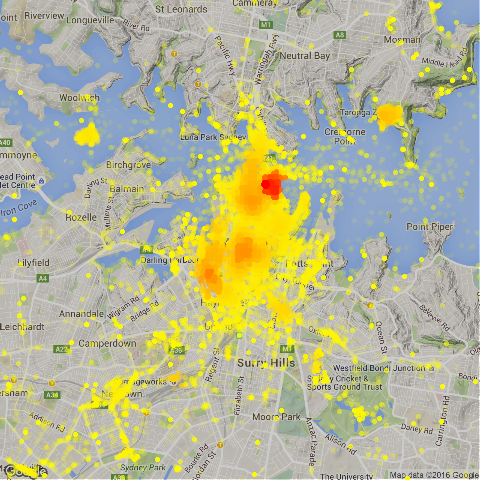Point Density Plot of Australia	Point Density Plot of Sydney

Introducing Interactive Maps with Leaflet

The leaflet package provides a great way to build interactive maps. These maps can be embedded into an html document (like on this website) or built into a Shiny application. Leaflet interactive geospatial graphics are very customizable, and can handle 50-100K points before slowing down. Below is a heatmap of the Sydney Flickr Data using the Point Density output. The code below is the basic and simplest command to generate a leaflet map.

leaflet(data=sydney) %>% 
  addTiles() %>% addMarkers(~lon, ~lat
)

Answering questions with data

Now lets start seeing what kind of questions we could ask and answer with the Flickr Data:

• Can I understand events with this data?
• Can I understand movement with this data?

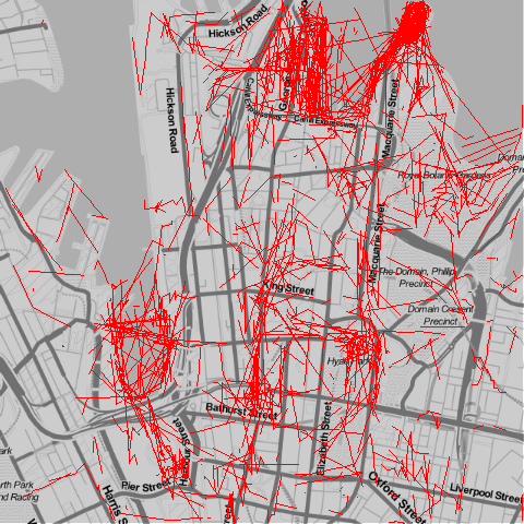
Can I understand movement with this data?

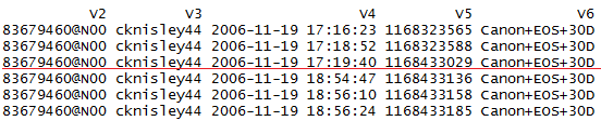
For this blog, let’s take a look at understandning movement with the Flickr Data. Oftentime these photos are created by tourists who are taking multiple pictures. Given that many photographs are taken while walking (as opposed to taken through the window of a car), we can assume some of these series of pictures are captured by a walking tourist. If we link pictures that were taken in close temporal proximity by the same photographer, then we can build “tracks” of where these photographers moved. By putting all of these tracks together, we can gain an understanding of movement in a city (in this case, Sydney). To accomplish this, I create a subset of photos shot by a single photographer, order by time, establish break points when the difference in tims is greater than 8 minutes, establish group labels, and then visualize with ggmap. The main portion of the code as well as the visualization are provided below.

photographers<-unique(sydney$V2)              #ID photographers
final<-list()                                 #Create OJB to store results
for(i in 1:length(photographers)){            
temp<-subset(sydney,V2==photographers[i])     #Subset by photographer
temp<-temp[order(temp$V4),]                   #Order by time
breakpoints <- c(FALSE,diff(temp$V4)>8*60)    #Establish break points if diff > 8min
temp$label <- as.numeric(cut.POSIXt(temp$V4, c(min(temp$V4), 
              temp[breakpoints, "V4"], max(temp$V4)+1)))    #Convert factor to label
temp$label<-paste(temp$V2,temp$label,sep="")  #Concatenate label with username
final[[i]]<-temp                              #Store temp data
}
final<-do.call("rbind", final)                #Convert from list to dataframe

Flickr Tracks	Understanding the Algorithm

Crowd sourcing event planning: Best Place to Watch Fireworks