A week or so ago I shared a blog demonstrating how to download reputable COVID-19 data and generate temporal Coronavirus case count plots like the ones seen in top news sites such as the New York Times or Wall Street Journal. This week I will walk through how to use that same data from last week and the R programming language to generate a choropleth plot by county in the United States.

As the COVID-19 virus wreaks havoc across our world, many of us are sitting in our homes trying to figure out if there’s something we can do to help. Many of those with medical skills have already responded to calls for help. Some of us with experience in the data science fields have tried to figure out if there’s something we can do. I am pretty late to the game to work on this, but still wanted to start from scratch. Part of my interest in starting from scratch is that I’ve found that you don’t fully understand a problem unless you really dive in and play with the data. This project gave me the opportunity to to that. If you want to look at some folks that are ahead of me, I recommend this blog post

Backup is an important aspect of data security. Users create backups of physical or cloud based machines and data just in case some unforeseen accident should occur. Several notable backup solutions are available, to include Apple’s Time Machine, Windows 10 File History, and Ubuntu Backups.

The secret sauce to a good backup solution is to make incremental snapshots of any file that has changed, while not duplicating files that haven’t changed. The easiest way to do this is with hard links to unchanged files. Hardlinks allow a user to save files once, have incremental snapshots of their entire machine or directory, and then to only fully delete a file when the final hard link is severed.

Bash Time Machine Code

In the code below, I illustrate how to do this with a very simple bash script. This script can be deployed in the terminal on Mac or Ubuntu or in Windows Subsystem for Linux (WSL). I recommend only using this script as a backup solution if you’re fairly knowledgeable about bash scripting and understand hard links.

#!/bin/sh
date=`date "+%Y%m%d%H%M%S"`
rsync -aPW --link-dest=/backup_drive/Backups/current --exclude=".*/"  --exclude-from='exclude_me.txt'  /directory/to/backup  /backup_drive/Backups/back-$date
rm -f /backup_drive/Backups/current
ln -s back-$date /backup_drive/Backups/current

This code is a collection of code that I used for scraping images from a variety of locations (Google images, Flickr, Tumblr, Twitter, and Instagram). I used these platforms to collect images for training a Convolutional Neural Network model. In my case I was building a CNN to detect internet memes, and used the platforms above to get ~20K examples of memes (and ~20K non-meme images).

I’ve had an opportunity to work on a variety of open source social media projects. A number of these have involved Twitter Data. Having worked extensively with Twitter Data in R, I migrated to Python in 2017. This migration was done for several reasons. First, I discovered that if you don’t extract the raw JSON data for Twitter (which many R packages don’t), then you end up dropping alot of valuable data on the floor. Additionally, most third party applications require the full Twitter JSON payload. Once you do decide to collect raw JSON, it makes sense to transition to Python because of the ease of working with JSON data in Python (JSON data easily transitions to a Python dictionary). You can work with JSON data in R (usually in a list of lists), but (in my opinion) it is not as easy or straightforward.

Many type of publicly available information, particularly social media, contain various languages. In addition to conducting machine translation, it is often helpful to simply identify the language. The cldr package allows users to leverage the Google Chrome language identification algorithm. This package is by far the fastest language identification package that I have found for R.

Installing CLDR

cldr is no longer on CRAN, but archive source files are available. To install cldr, run the following code:

#install from archive
url <- "http://cran.us.r-project.org/src/contrib/Archive/cldr/cldr_1.1.0.tar.gz"
pkgFile<-"cldr_1.1.0.tar.gz"
download.file(url = url, destfile = pkgFile)
install.packages(pkgs=pkgFile, type="source", repos=NULL)
unlink(pkgFile)
# or devtools::install_version("cldr",version="1.1.0")

#usage
library(cldr)
demo(cldr)

As the size of data in our world continues to grow, we will increasingly have to deal with data that that doesn’t fit into memory (a constraining factor for those using R/Python). While one solution is to buy more RAM (which is now easier than ever in cloud services like Amazon Web Services and Azure), this is many times not feasible. In these cases, we need a storage solution to throw our data into and from which we can easily query. This query may be for traditional analysis in R/Python or it may be a query that feeds a Shiny application.

This blog is meant to walk an analyst through setting up an ELK stack in AWS. I have recently set up and extensively used an ELK stack in AWS in order to query 20M+ social media records and serve them up in a Kibana Dashboard. While AWS does offer Amazon Elastic Search Sevice, this service uses an older version of elasticsearch. I preferred to build it myself from the ground up so that I could customize the configuration to my needs. This tutorial is the result of hours of time on Google stitching together numerous blogs on the subject of ELK stacks. Note that this tutorial assumes that you have a basic knowledge of using AWS and the Linux terminal (for Linux basics, see Paul Gellerman’s DSCOE blog here)

Why Elasticsearch, Logstash, and Kibana?

Below are some solutions that I’ve used/explored:

1. SQLite (easy to set up and query with SQL commands, but some queries can take a while)
2. Unix Commands (if your data is in numerous CSV files, sometimes using grep from a Linux/Mac terminal can effectively query your data)
3. Apache Drill (this is a new tool that shows alot of promise for linux users. I haven’t used it yet, but Apache Drill seems like a great concept with a Schema-free SQL that can query Hadoop, NoSQL, and Cloud Storage. The use case that I’m exploring is using it to quickly query multiple JSON files sitting in AWS S3 Storage)
4. Elasticsearch: Elasticsearch (ES) is the core of the ELK Stack (Elasticsearch, Logstash, and Kibana). While not as easy to set up as SQLite, Elasticsearch uses blazing fast search for query. You can set it up on your laptop or single AWS node to query GBs of data, or you can set it up on hundreds of servers to query Petabytes of data.

Set up AWS Node

DO NOT setup an AWS AMI that is preconfigured (i.e. do not use popular the R/RStudio AMI that Louis Aslett maintains) because the RStudio webserver connection will impact the useability of the Kibana Dashboard. Instead, choose a basic Ubuntu Server AMI as seen below:

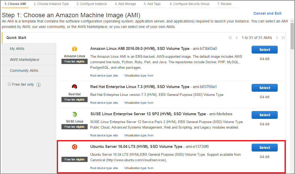
After choosing this, continue through the following steps:

1. Choose desired instance size (from my experience ES requires a minimum of 2 GB of RAM)
2. Leave instance detail default settings
3. Increase EBS storage if desired (this is essentially the size of your hard drive…you can get up to 30GB on the free tier)
4. Adjust Security Group by adding HTTP and HTTPS and restricting source IP as desired
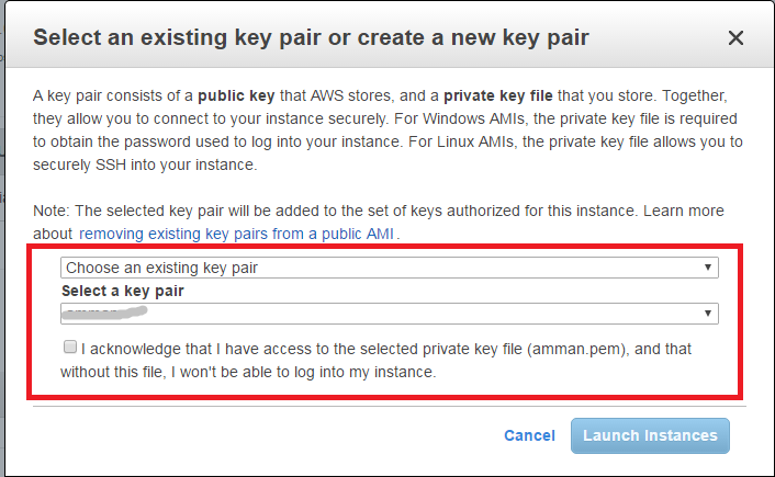
5. Make sure you create and select a key pair (see below) in order to later connect to your node through SSH protocol

As a side note, to save money ensure you power off you nodes when not in use. As you can see from this blog it isn’t necessarily easy to set up an ELK stack, and once you set it up you don’t necessarily want to terminate it, but if you stop it you will only pay for storage space and not for compute time.

Java

Now that you have an AWS instance up and running, let’s connect and start configuring your bare bones Ubuntu node. You can connect through SSH protocol using Putty (Windows 7), Bash shell (Windows 10) or standard terminal on Linux/Mac. For those that are new to SSH, use the command below to connect with a key pair:

ssh  -i  path-to-key/key  ubuntu@ip.address

Now that you have connected to your Ubuntu node, check for updates and install updates with the following lines of code (note: you will have to copy and paste each line separately):

sudo apt-get update
sudo apt-get upgrade

Now let’s install java with the following lines (once again, if you’re using copy/paste, remember that you will have to copy/paste each line separately)

sudo add-apt-repository -y ppa:webupd8team/java
sudo apt-get update
echo debconf shared/accepted-oracle-license-v1-1 select true | sudo debconf-set-selections
echo debconf shared/accepted-oracle-license-v1-1 seen true | sudo debconf-set-selections
sudo apt-get -y install oracle-java8-installer
java -version

Your last line should produce a result that looks something like this:

java version "1.8.0_111"
Java(TM) SE Runtime Environment (build 1.8.0_111-b14)
Java HotSpot(TM) 64-Bit Server VM (build 25.111-b14, mixed mode)

Elasticsearch

Now we’ll install elastic search with the following lines of code. This is downloading the package directly from elastic.co and installing it.

wget -qO - https://packages.elastic.co/GPG-KEY-elasticsearch | sudo apt-key add -
  echo "deb http://packages.elastic.co/elasticsearch/2.x/debian stable main" | sudo tee -a etc/apt/sources.list.d/elasticsearch-2.x.list
sudo apt-get update && sudo apt-get install elasticsearch
sudo update-rc.d elasticsearch defaults 95 10  ##This starts ES on boot up
sudo /etc/init.d/elasticsearch start        
curl 'http://localhost:9200'

Now we need to configure ES to restrict access. To do this, we will open the configuration file in a command lind text editor:

sudo nano /etc/elasticsearch/elasticsearch.yml

and change the network host to localhost.:

network.host: localhost

If you’ve installed this correctly, the last line should generate the something that looks simlar to:

{
  "name" : "Stonewall",
  "cluster_name" : "elasticsearch",
  "cluster_uuid" : "Lz_jcK-IQXuVrbBrcHOA7w",
  "version" : {
    "number" : "2.4.3",
    "build_hash" : "d38a34e7b75af4e17ead16f156feffa432b22be3",
    "build_timestamp" : "2016-12-07T16:28:56Z",
    "build_snapshot" : false,
    "lucene_version" : "5.5.2"
  },
  "tagline" : "You Know, for Search"
}

Logstash

Logstash is “an open source, server-side data processing pipeline that ingests data from a multitude of sources simultaneously, transforms it” and sends it to your ES engine. While not necessary to use ES, it does provide a convenient way to load data if desired (especially if you’re unsure of how to create an elastic search mapping).

echo "deb https://packages.elastic.co/logstash/2.3/debian stable main" | sudo tee -a /etc/apt/sources.list
sudo apt-get update && sudo apt-get install logstash
sudo update-rc.d logstash defaults 95 10  ##This starts logstash on startup
sudo /etc/init.d/logstash start

Kibana

Kibana is an open source dashboard that will easily visualize data held in your ES Stack. Install Kibana with the code below:

echo "deb http://packages.elastic.co/kibana/4.5/debian stable main" | sudo tee -a /etc/apt/sources.list
sudo apt-get update && sudo apt-get install kibana
sudo update-rc.d kibana defaults 95 10

Open the Kibana configuration vile for editing:

sudo nano /opt/kibana/config/kibana.yml

In the configuration file, arrow down to the line that specifies server.host, and replace the IP address (default is “0.0.0.0”) with

server.host: "localhost"

NGINX

Now we’ll install Nginx in order to set up a reverse proxy.

sudo apt-get install nginx apache2-utils

We will use htpasswd to create an admin user (in the following code, change “kibanaadmin” to another name)

sudo htpasswd -c /etc/nginx/htpasswd.users kibanaadmin

Enter a password at the prompt.

Now we will set the Nginx default server block by copying creating the following file:

sudo nano /etc/nginx/sites-enabled/nsm

and then copying the code below, ensuring that you copy and paste your AWS URL in to replace the one I’m using here:

server {
  listen 80;

  server_name ec2-54-166-151-27.compute-1.amazonaws.com;

  auth_basic "Restricted Access";
  auth_basic_user_file /etc/nginx/htpasswd.users;

  location / {
    proxy_pass http://localhost:5601;
    proxy_http_version 1.1;
    proxy_set_header Upgrade $http_upgrade;
    proxy_set_header Connection 'upgrade';
    proxy_set_header Host $host;
    proxy_cache_bypass $http_upgrade;
  }
}

Now run the code below to restart Nginx:

sudo /etc/init.d/nginx restart

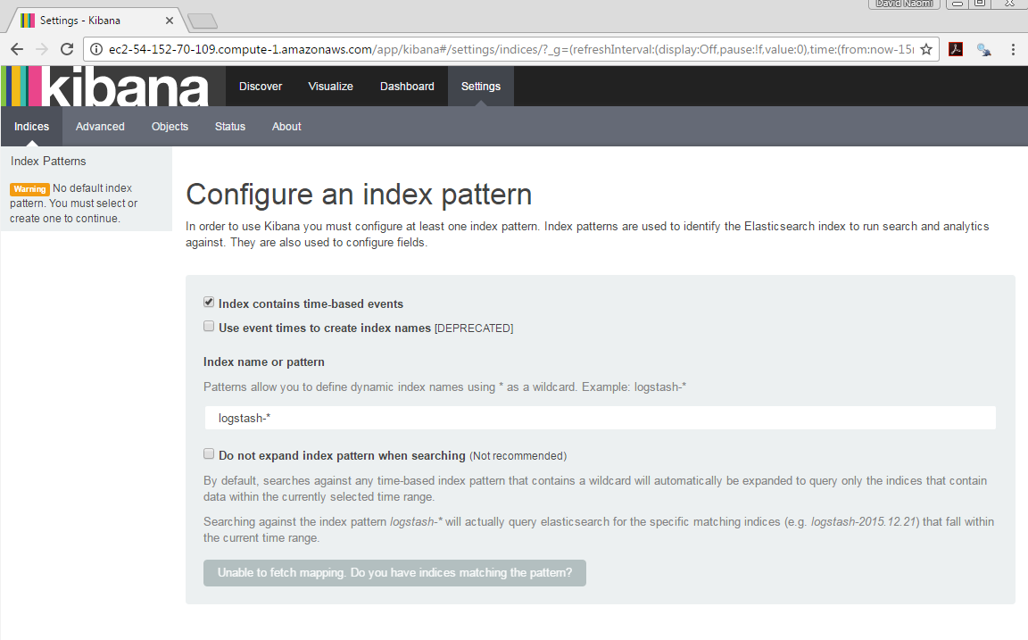
At this point, reboot your AWS and node and then put your AWS Public DNS in a browser. You should be prompted for the username and password that you used above. After entering this, you should get a screen that looks like:

If you run into any problems, below are several commands that I found helpful:

##Restart Nginx
sudo service nginx restart

##Restart ES
sudo /etc/init.d/elasticsearch restart

##Restart Kibana
sudo service kibana start

Now, we need to load some data into ES. The easiest way is to load JSON data from Python. The elastic packages exists for R that can assist in loads some data. For my purposes, I chose to use Logstash to load Twitter Data from large CSV files. I created a new file in my home directory called myTweet.conf, and put the following mapping in this configuration file (note that I’m loading data that I scraped from the Twitter API and enriched with City, Country, and Language fields).

input {
    file {
        path => "/home/ubuntu/Dropbox/load/TwitterData2016-11-07.csv"
        type => "twitter"
        start_position => "beginning"
    }
}

filter {
    csv {
        columns => [    "text" ,
                         "favorited" ,
                         "favoriteCount",
                         "replyToSN" ,
                         "created" ,     
                         "truncated" ,  
                         "replyToSID" ,
                         "id"   ,
                         "replyToUID" ,
                         "statusSource" ,
                         "screenName"  ,
                         "retweetCount",
                         "isRetweet"  ,
                         "retweeted" ,
                         "longitude" ,
                         "latitude" ,
                         "language" ,
                         "city",
                         "country"]
        separator => ","
        remove_field => ["replyToSN","truncated","replyToSID","replyToUID"]
    }
    date {
        match => ["created", "YYYY-MM-dd HH:mm:ss"]
        timezone => "America/New_York"
        target => "created"
    }

    mutate {
        convert => {
        "text" => "string"
           "favoriteCount"  => "integer"
            "id" => "integer"
             "statusSource" => "string"
                "screenName" => "string"
                "retweetCount" => "integer"
                "isRetweet" => "boolean"
                "retweeted"  => "boolean"
                 "longitude" => "float"
                 "latitude" => "float"
                 "language" => "string"
                "city" => "string"
                "country" => "string"
        }
    }
}

output {
    elasticsearch {
        action => "index"
        hosts => "127.0.0.1:9200"
        index => "tweets_20161215"
    }
}

Note that by using “tweets_date” for an index name, I can use a wildcard (*) in Kibana and then delete indices in order to allow the data to age off the stack.

To load a file using this mapping, run the following command in terminal (run this command for each CSV file you put into myTweet.conf):

 /opt/logstash/bin/logstash -f ~/myTweet.conf

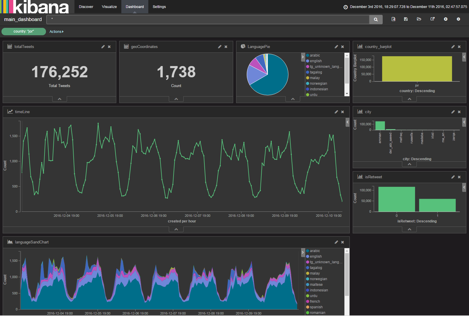
At this point, I’ve loaded over 20 million records (tweets) into my ES, and the below Kibana dashboard has been very responsive (I usually wait 5 seconds for queries, compared to 10 minutes with Sqlite).

Finally, here’s a couple of commands that are helpful:

## List ES indices (with number of records and size on disk)
curl 'localhost:9200/_cat/indices?v'

## Delete an Index
curl -XDELETE 'http://localhost:9200/tweets_20161226/'

If you have any suggestions or questions, please reach out at david.m.beskow.mil@mail.mil.

A little while back I had the opportunity to help Paul Evangelista convert his point density algorithm from perl to R. This is a novel algorithm that he developed to help visualize point data in a combat environment. He found that military leaders preferred to have a heat map that still maintained the fidelity of the original point data (whereas most kernel density algorithms ‘spread’ the density around, and in the process tend to lose the point data granularity). This algorithm is useful for any event data, to include military, criminal, natural disaster, or spatial social media (i.e. Flickr Photos). I’ve provided an example of using this algorithm below, and have included the code for those who want to dig into it.

The Global Knowledge Graph, related to the Global Database of Events, Language, and Tone, provides a very rich dataset with many potential use cases. In this blog I will illustrate how we used it to identify influencers in a national or regional network. This algorithm feeds a Shiny WebApp located here. The basic idea of this algorithm is to subset 30 days of GKG data based on regions (we found that national capitals worked best), build a network of the people in this subset (based on co-mentions), and then to run network centrality algorithms against this network to order the data based on influence. The top influencers on this list are then fused with Wikipedia data in order to provide a two sentence description.

In this blog I will explore some geospatial analysis and visualization using the Flickr Data found in the Creative Commons 100M Images/Video. In particular I will demonstrate Paul Evangelista’s Point Density plotting package as well as the leaflet interactive map package. I originally created this as part of an RStudio Presentation that I presented at the Army’s Data Science Center of Education (DSCOE). I’ve extracted this part of it for a blog post.

I’ve wanted to spend some time to learn how to use the grid graphics pattern for a while. A recent assignment at work gave me the opportunity to do so. I found a great tutorial by Zhou and Braun entitled Fun with the R Grid Package. The grid package allows you to build up a visualization from the ground up. By using viewports, the user can define any piece of the canvas in order to build a small visualization. The power of these visualization comes together when many of these smaller visualizations are put together.

In summary, this post will demonstrate four methods for reverse geocoding. These three methods are summarized below: