
Point Density Algorithm
A little while back I had the opportunity to help Paul Evangelista convert his point density algorithm from perl to R. This is a novel algorithm that he developed to help visualize point data in a combat environment. He found that military leaders preferred to have a heat map that still maintained the fidelity of the original point data (whereas most kernel density algorithms ‘spread’ the density around, and in the process tend to lose the point data granularity). This algorithm is useful for any event data, to include military, criminal, natural disaster, or spatial social media (i.e. Flickr Photos). I’ve provided an example of using this algorithm below, and have included the code for those who want to dig into it.
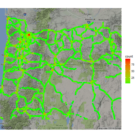
The algorithm uses a grid (parameterized by distance between grid lines) to speed up computations, and uses a radius to identify local neighborhoods where an event adds density. In the example below, we use the algorithm to generate a heat map of simulated event data along the Oregon highway system.
Example with Simulated Event data in Oregon
The data is 80,000 events with a simple lat, lon, and timestamp. This dataset was randomly created along the Oregon highway system. Here’s what the data looks like:
library(pointdensityP)
head(Arigon)   ##Arigon is included in the pointdensityP package

##   longitude latitude       date
## 1 -124.0799 44.47140 2011-10-17
## 2 -121.3318 44.05141 2012-03-06
## 3 -120.1861 45.23710 2012-11-09
## 4 -122.5620 45.55909 2011-08-06
## 5 -117.9159 45.56549 2012-08-23
## 6 -118.9329 44.41495 2012-07-28
Here’s how apply the pointdentiy algorithm against this data set. In this case, we’ve found that a grid_size of 1 km and a radius of 2 km is appropriate.
Here’s what Arigon Density Data looks like now:
head(Arigon_density)

##           lat       lon     count dateavg
## 91   43.68960 -117.0918 0.0794503   15561
## 485  43.80316 -120.5646 0.0794503   15204
## 793  44.14196 -117.4040 0.0794503   15164
## 976  43.70740 -122.2894 0.0794503   15454
## 1195 45.01085 -118.9954 0.0794503   15552
## 1408 43.21195 -123.2440 0.0794503   15521
Now we will visualize the data using the ggmap package.
library(ggmap)
map_base <- qmap(location="44.12,-120.83", zoom = 7, darken=0.3)
map_base + geom_point(aes(x = lon, y = lat, colour = count),
                      shape = 16,
                      size = 2,
                      data = Arigon_density) +
          scale_colour_gradient(low = "green", high = "red")
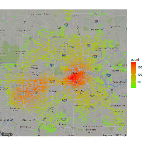
Example with Crime Data in Houston
Here’s another example using crime data from Houston. This is using data from the ggmap package that we’ve cleaned and included in the pointdensityP package.
H_crime <- pointdensity(df = clean_crime,
                        lat_col = "lat",
                        lon_col = "lon",
                        grid_size = 1,
                        radius = 4)

map_base <- qmap(location="29.76,-95.42", zoom = 11, darken=0.3)
map_base +
  geom_point(aes(x = lon, y = lat, colour = count),
             shape = 16,
             size = 1,
             alpha=0.2,
             data = H_crime) +
  scale_colour_gradient(low = "green", high = "red")
You can also see how I used this algorithm to visualize Flickr data at this blog
The full algorithm is given below:
pointdensity <- function (df, lat_col, lon_col, date_col = NULL, grid_size, radius) {
    grid_size <- round(grid_size/111.2, digits = 3)
    rad_km <- radius
    rad_dg <- rad_km/111.2
    rad_steps <- round(rad_dg/grid_size)
    rad_km <- rad_steps * grid_size * 111.2
    cat("\nThe radius was adjusted to ", rad_km, "km in order to accomodate the grid size\n\n")
    cat("algorithm grid step radius is ", rad_steps, "\n\n")
    radius <- rad_steps
    h <- new.env(hash = TRUE)
    avg_date <- new.env(hash = TRUE)
    bh <- new.env(hash = TRUE)
    b_date <- new.env(hash = TRUE)
    lat_data <- df[, lat_col]
    lat <- lat_data * (1/grid_size)
    lat <- round(lat, 0)
    lat <- lat * (grid_size)
    lon_data <- df[, lon_col]
    lon <- lon_data * (1/grid_size)
    lon <- round(lon, 0)
    lon <- lon * (grid_size)
    if (is.null(date_col)) {
        date <- rep(0, length(lon))
    }
    if (!is.null(date_col)) {
        date <- as.Date(df[, date_col])
        date <- as.numeric(date)
    }
    key.vec <- paste(lat, lon, sep = "-")
    data_length <- length(lat)
    ulat <- c()
    ulon <- c()
    cat("binning data...\n\n")
    pb <- txtProgressBar(title = "point density calculation progress",
        label = "0% done", min = 0, max = 100, initial = 0, style = 3)
    for (i in 1:data_length) {
        key <- paste(lat[i], lon[i], sep = "-")
        if (is.null(h[[key]])) {
            bh[[key]] = 1
            h[[key]] = 1
            b_date[[key]] = date[i]
            avg_date[[key]] = b_date[[key]]
            ulat <- c(ulat, lat[i])
            ulon <- c(ulon, lon[i])
        }
        else {
            bh[[key]] <- bh[[key]] + 1
            h[[key]] <- bh[[key]]
            b_date[[key]] = b_date[[key]] + date[i]
            avg_date[[key]] = b_date[[key]]
        }
        setTxtProgressBar(pb, i/(data_length) * 100, label = info)
    }
    cat("\n", "Data length is ", data_length, "; reduced to ",
        length(ulat), "bins. Density calculation starting.\n\n")
    lat <- ulat
    lon <- ulon
    pb <- txtProgressBar(title = "point density calculation progress",
        label = "0% done", min = 0, max = 100, initial = 0, style = 3)
    counter <- 0
    data_length <- length(lat)
    pb2 <- txtProgressBar(title = "point density calculation progress",
        label = "0% done", min = 0, max = 100, initial = 0, style = 3)
    for (i in 1:data_length) {
        counter <- counter + 1
        if (counter > 99) {
            flush.console()
            counter <- 0
        }
        ukey <- paste(lat[i], lon[i], sep = "-")
        lat.vec <- seq(lat[i] - radius * grid_size, lat[i] +
            radius * grid_size, grid_size)
        for (lat.temp in lat.vec) {
            t <- sqrt(round(((radius * grid_size)^2 - (lat.temp -
                lat[i])^2), 8))
            t <- t/cos(lat.temp * 2 * pi/360)
            t <- t/grid_size
            t <- round(t, 0)
            t <- t * grid_size
            lon.vec <- seq(lon[i] - t, lon[i] + t, grid_size)
            for (lon.temp in lon.vec) {
                key <- paste(lat.temp, lon.temp, sep = "-")
                if (is.null(h[[key]])) {
                  h[[key]] = bh[[ukey]]
                  avg_date[[key]] = b_date[[ukey]]
                }
                else {
                  if (key != ukey) {
                    h[[key]] <- h[[key]] + bh[[ukey]]
                    avg_date[[key]] = avg_date[[key]] + b_date[[ukey]]
                  }
                }
            }
        }
        info <- sprintf("%d%% done", round((i/data_length) *
            100))
        setTxtProgressBar(pb2, i/(data_length) * 100, label = info)
    }
    close(pb)
    count_val <- rep(0, length(key.vec))
    avg_date_val <- rep(0, length(key.vec))
    for (i in 1:length(key.vec)) {
        count_val[i] <- h[[key.vec[i]]]
        avg_date_val[i] <- avg_date[[key.vec[i]]]/count_val[i]
        count_val[i] <- count_val[i]/(pi * rad_km^2)
    }
    final <- data.frame(lat = lat_data, lon = lon_data, count = count_val,
        dateavg = avg_date_val)
    final <- final[order(final$count), ]
    return(final)
    cat("done...\n\n")
}