
Four Methods for Reverse Geocode
In summary, this post will demonstrate four methods for reverse geocoding. These three methods are summarized below:
- ggmap reverse geocoding function
- Extract country and state/province data from shapefile
- Identify closest city
- Identify closest zip code (US Only)
In my years of munging geospatial data, I’ve run into a number of instances when I have a data set with a lat-lon combination, but no other spatial reference (i.e. Country, State/Province, City, etc.). If you have a data set with latitude and longitude but not Country, State/Province, or city, than I’d recommend using one of the methods below (or a combination of them) to add a Country, State/Province, and/or City field to your data. The easiest of these to use is the reverse geocoding function from the ggmap package. This is very easy to use and fairly accurate. However, it is rate limited at 2500 reverse geocodes daily, and can take up to 45 minutes to reverse geocode 2500 lat/lon combinations (depending on internet connection). Additionally, you will not be able to use this function from an air-gapped network or from an austere location with limited internet connectivity. The last three methods work must faster, are not rate limited, and can work in an air-gapped network (or otherwise austere environment). In these cases, if you have US Only spatial data, I’d recommend using the zip code method below. If you have international data, and require Country and State/Province, use the shapefile data extraction method. If you require Country and City data, use the world city data in the second method. If you require Country, State/Province, and City data, you will have to use a combination of both the shapefile data extraction and international city data methods.
Using the revgeocode function
The revgeocode method from the ggmap package package is intuitive and easy to use. An example is given below:
First, let’s establish some random cities to use as an example:
## Choose random cities to test our algorithms
cities <- data.frame(
  lat=c(-33.86785,51.50726,55.75,39.90750,35.46756,-1.28333,52.52330,-22.90278),
  lon=c(151.20732,-0.1278328,37.5,116.39723,-97.51643,36.81667,13.41377,-43.2075)
)
Extract Data from Shapefile
This method will extract spatial data from a shapefile. This is most often conducted to enrich your original data with Country and State/Province data. This method is the most accurate method for adding country and state/province since it uses point-in-polygon calculations. The shapefile data is also usually more accurate than the city data used in the next example.
To manipulate shapefiles, we first need to load the sp and maptools packages.
library(sp)
library(maptools)
Next you will need to download a Level 1 World Shapefile. I’ve found a decent shapefile that Harvard maintains at the following link: Harvard Level 1 World Shapefile.
After downloading and unzipping the shapefile, we read it into our environment below:
world.shp <- readShapePoly("g2008_1.shp")
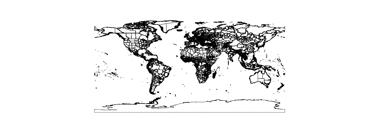
proj4string(world.shp) <- CRS("+proj=longlat +ellps=WGS84")This is what our Level 1 shapefile looks like (remember that Level 1 Shapefiles are one level below country boundary for all countries).
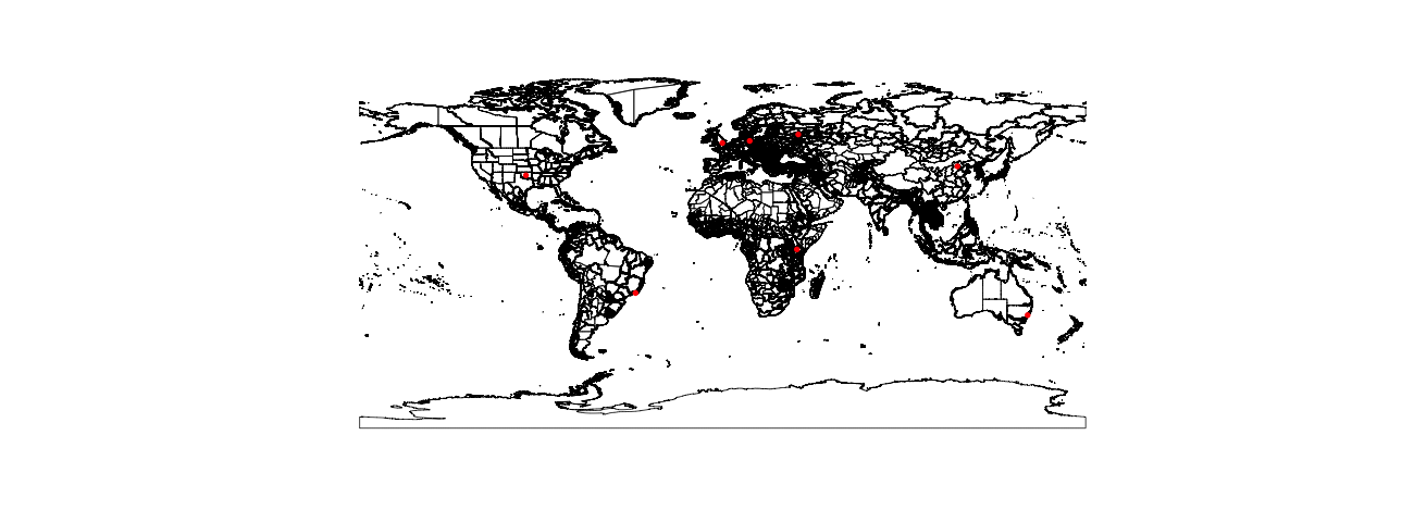
Now I’m going to read in a list of lat/lon combinations from around the world to test our code on. While these aren’t explicitly named, note that they were created by geocoding the following cities: Sydney, London, Moscow, Beijing, Oklahoma City, Nairobi, Berlin, and Rio de Janero.
## Choose random cities to test our algorithms
cities <- data.frame(
  lat=c(-33.86785 , 51.50726 , 55.75000 , 39.90750 , 35.46756 , -1.28333 , 52.52330 ,-22.90278),
  lon=c(151.20732 , -0.1278328 , 37.5 ,116.39723 ,-97.51643  ,36.8166700 , 13.41377, -43.2075)
)
Now let’s see a picture of our cities plotted over our shapefile:
Next, we need to convert the cities data frame to a Spatial Points Data Frame. We start by creating a separate object called cities.sp, and then creating the Spatial Points Data Frame.
cities.sp <- cities                              ## Rename
coordinates(cities.sp) <- ~lon+lat               ## Create Spatial Points Data Frame
proj4string(cities.sp) <- CRS("+proj=longlat +ellps=WGS84")
Next we will use point-in-polygon calculations to determine which polygon each point fall in. The over command in R is a powerful command that allows us to conduct this point-in-polygon calculation.
## Conduct point-in-polygon calculation and extract data
extracted.data <- over(cities.sp,world.shp)

extracted.data
## AREA PERIMETER G2008_1_ G2008_1_ID ADM1_CODE ADM0_CODE
## 1 76.60676282 78.223011 32966 32965 470 17
## 2 17.22851535 50.129004 9630 9629 3182 256
## 3 0.14140157 1.653553 9584 9583 2535 204
## 4 1.73808134 7.161621 13166 13165 899 53
## 5 18.00501971 25.756017 14010 14009 3250 259
## 6 0.05658006 1.664051 27161 27160 51328 133
## 7 0.11789101 2.070110 10602 10601 1310 93
## 8 3.83091826 21.150444 32532 32531 683 37
## ADM0_NAME ADM1_NAME
## 1 Australia New South Wales
## 2 U.K. of Great Britain and Northern Ireland England
## 3 Russian Federation Moskva
## 4 China Beijing Shi
## 5 United States of America Oklahoma
## 6 Kenya Nairobi
## 7 Germany Berlin
## 8 Brazil Rio De Janeiro
## LAST_UPDAT CONTINENT REGION STR_YEAR0 STR_YEAR1
## 1 20050415 Oceania Australia and New Zealand 0 0
## 2 20050825 Europe Northern Europe 0 0
## 3 20050415 Europe Eastern Europe 0 0
## 4 20050415 Asia Eastern Asia 0 0
## 5 20060103 Americas Northern America 0 0
## 6 20081111 Africa Eastern Africa 0 0
## 7 20051229 Europe Western Europe 0 0
## 8 20050415 Americas South America 0 0
## EXP_YEAR0 EXP_YEAR1
## 1 0 0
## 2 0 0
## 3 0 0
## 4 0 0
## 5 0 0
## 6 0 0
## 7 0 0
## 8 0 0Next we will merge this data with our original data:
## Merge Data
cities$Country <- extracted.data$ADM0_NAME
cities$level_1 <- extracted.data$ADM1_NAME
Below is our final data frame.
| lat | lon | Country | level_1 | |
|---|---|---|---|---|
| 1 | -33.87 | 151.21 | Australia | New South Wales |
| 2 | 51.51 | -0.13 | U.K. of Great Britain and Northern Ireland | England |
| 3 | 55.75 | 37.50 | Russian Federation | Moskva |
| 4 | 39.91 | 116.40 | China | Beijing Shi |
| 5 | 35.47 | -97.52 | United States of America | Oklahoma |
| 6 | -1.28 | 36.82 | Kenya | Nairobi |
| 7 | 52.52 | 13.41 | Germany | Berlin |
| 8 | -22.90 | -43.21 | Brazil | Rio De Janeiro |
Now we have spatial data added to our original data frame and we can easily bin data by country or province.
Reverse Geocode to City Level (with OpenGeoCode Data)
The next method I’ll demonstrate is to find the nearest world city. There are several data bases available online for doing this. Open Geo Code maintains a database at the following link. This database is maintaned by the National Geospatial Agency (NGA) and is fairly comprehensive. It does contain multiple entries for each city (usually to capture various spellings of the same city). My biggest complaint of this data set is that it does not contain any cities for the US or China. While I can sort of understand not having any US cities, I have no idea why it does not contain Chinese cities.
The other data set that I’ve used before is from Maxmind link. This data set is not maintained as much as the NGA data set, but does contain all countries (to include US cities). This is a fairly large dataset, containing over 3 million entries.
Both data sets require some cleaning. The NGA dataset contains a unique feature ID, which can be used to remove duplicates. Ensure that you maintain either an english or latin spelling of city names. The Maxmind data set does not contain a unique feature ID, so I had to create one by concatenating the lat/lon combination.
With Maxmind Data
For this blog post, I will only demonstrate using the Maxmind data. First we’ll read in the data:
world.cities <- read.csv("worldcitiespop.txt",as.is=TRUE)Next we will concatenate the lat/lon combination in order to create a unique identifier. Having done this, we remove duplicates:
## Create identifier with lat/lon
world.cities$id<-paste(world.cities$Latitude,world.cities$Longitude,sep="")

## Remove Duplicates
world.cities <- world.cities[!duplicated(world.cities$id),]
Next, we will use the fields package to create a distance matrix, and then choose the closest city to each of these grids. Note that if you have grids near borders, this algorithm may find that the closest city is on the other side of the border.
library(fields)

## Create distance matrix
mat<-rdist.earth(data.matrix(cities[,c(2,1)]),data.matrix(world.cities[,c(7,6)]))

## Add fields to data frame
cities$country <- NA
cities$city <- NA
cities$accent_city <- NA
cities$dist <- NA

## Loop through data frame and find closes city, merging country and level 1 data
for(i in 1:nrow(cities)){
k<-which.min(mat[i,])
cities$country[i] <- world.cities$Country[k]
cities$city[i] <- world.cities$City[k]
cities$accent_city[i] <- world.cities$AccentCity[k]
cities$dist[i] <- mat[i,k]
}
Now that this is done, we can print our new data frame to see how it worked.
| lat | lon | country | city | accent_city | dist | |
|---|---|---|---|---|---|---|
| 1 | -33.87 | 151.21 | au | pyrmont | Pyrmont | 0.43 |
| 2 | 51.51 | -0.13 | gb | charing cross | Charing Cross | 0.25 |
| 3 | 55.75 | 37.50 | ru | shelepikha | Shelepikha | 0.65 |
| 4 | 39.91 | 116.40 | cn | beijing | Beijing | 1.55 |
| 5 | 35.47 | -97.52 | us | oklahoma city | Oklahoma City | 0.02 |
| 6 | -1.28 | 36.82 | ke | nairoba | Nairoba | 0.00 |
| 7 | 52.52 | 13.41 | de | berlin | Berlin | 0.74 |
| 8 | -22.90 | -43.21 | br | praia formosa | Praia Formosa | 0.16 |
Reverse Geocode US Zipcodes
The reverse Geocode of US Zipcodes is very similar to the world cities algorithm. Note that this data frame can also be used to geocode data that has a zip code but does not contain lat/lon. Several open source zip code data files are available online. The one that I’m going to use here was accessed at OpenGeoCode.
First, let’s read the data into our environment. Note that in this case, I explicitly declare the field types so that the zipcode field is read into R as a character field instead of of a numeric field (if read in as a numeric field, it will remove any leading zero’s).
zip <- read.csv("cityzip.csv" ,as.is=TRUE,
                colClasses = c("character","character","character","numeric","numeric","numeric"))
Here’s the list of US cities that we will use to test our algorithm. These lat/lon combinations represent the city center of Portland, Salt Lake City, Dallas, Knowxville, Oklahoma City, Orlando, Raleigh, and Boston.
us.cities <- data.frame(
  lat=c(45.50786 ,40.76078 ,32.78306 ,35.96064 ,35.46756 ,28.53834 ,35.88904 ,42.35843),
  lon=c(-122.69079,-111.89105,-96.80667,-83.92074 , -97.51643 , -81.37924,-82.83104  ,-71.05977)
)
Next we use an algorithm very similar to the world city algorithm to reverse geocode the lat/lon combinations.
library(fields)
mat<-rdist.earth(data.matrix(us.cities[,c(2,1)]),data.matrix(zip[,c(5,4)]))

us.cities$city <- NA
us.cities$postal <- NA
us.cities$dist <- NA

for(i in 1:nrow(us.cities)){
k<-which.min(mat[i,])
us.cities$city[i] <- zip$City[k]
us.cities$postal[i] <- zip$Postal[k]
us.cities$dist[i] <- mat[i,k]
}
Let’s check our final product:
| lat | lon | city | postal | dist | |
|---|---|---|---|---|---|
| 1 | 45.51 | -122.69 | Portland | 97201 | 0.45 |
| 2 | 40.76 | -111.89 | Salt Lake City | 84114 | 0.42 |
| 3 | 32.78 | -96.81 | Irving | 75202 | 0.04 |
| 4 | 35.96 | -83.92 | Knoxville | 37902 | 0.21 |
| 5 | 35.47 | -97.52 | Oklahoma City | 73102 | 0.55 |
| 6 | 28.54 | -81.38 | Orlando | 32801 | 0.89 |
| 7 | 35.89 | -82.83 | Hot Springs | 28743 | 0.23 |
| 8 | 42.36 | -71.06 | Boston | 02109 | 0.51 |